3.2 Object Types

Field, Array, and Group Objects implement sampled fields in Data Explorer. Additional Object types, used to construct models for rendering, are described in Appendix B. "Importing Data: File Formats".

Fields

Field Objects are the fundamental Objects in the Data Explorer data model. A Field represents a mapping from some domain to some data space. The domain of the mapping is specified by a set of positions and (generally) a set of connections that allow interpolation of data values for points in the domain between specified positions. The mapping at all points in the domain is represented implicitly by specifying data that are dependent on (located at) the sample points or on the connections between the sample points (cell-centered data).

This simple abstraction is sufficient for representing a wide range of things. For example, you can describe 3-dimensional volumetric data, whose domain is the region specified by the positions, and whose data space is the value associated with each position. Two-dimensional images have a domain that is the set of pixel locations, and a data space that consists of the pixel color. Two-dimensional surfaces imbedded in 3-space (that is, traditional graphical models) can have a domain that is the set of positions on the surface, and a data space that is, for example, the set of data values on that surface.

If the data are dependent on the given positions, then a data value at a point other than those given is found by interpolation within the connection in which the point resides. If the data is dependent on connections, then the data value is assumed to be constant within each connection. If no connections are specified, then there is no implied information about data values at positions other than those given.

The information in a Field is represented by some number of named components. Each component has a value, that is an Object. In general, components are Array Objects (described in more detail in the next section). For example, the "positions" component is an Array specifying the set of sample points; the "connections" component is an Array specifying a means to interpolate between the positions; and the "data" component is an Array specifying the data values.

Figure 2. Example of a Field Object

Figure 2 shows an example of a Field Object with four components. The "data" component specifies the user's data as an Array of data of arbitrary type (e.g., integer), which is dependent on (i.e., in one-to-one correspondence with) the "positions" component; the "positions" component specifies the sample points as an Array of 3-dimensional vectors; the "connections" component specifies a set of tetrahedra as vectors of four integers that refer to the "positions" component; and the "box" component lists the eight points that define the bounding box of the positions (i.e., of the Field itself). A complete list of defined component types is given in "Standard Components".

Field components (and Objects in general) can have attributes associated with them. For example, the "dep" attribute of a component records the dependency of that component on another component; thus the "data" component will have a "dep" attribute of "positions" or "connections," depending on whether the data are associated with the sample points or with the connections between them. A component can also have a "ref" attribute, indicating that it refers to another component. Typically, the "connections" component has a "ref" attribute of "positions," signifying that the items in the connections component refer to the positions component. A "connections" component must have an "element type" attribute naming the type of connections, such as "triangles", "quads", or "tetrahedra". A complete list of defined attributes is given in "Standard Attributes"; the complete list of element types is given in "Connections Component".

Note that Fields can share components. This allows, for example, several Fields to share the same positions and connections while having different data, colors, and so on. Figure 3 illustrates two such Fields that share 3-dimensional positions and tetrahedral connections, but each of which has separate (but still both position-dependent) data. The sharing is possible because the Arrays are Objects with a reference count stored in the Array header.

Figure 3. Shared Components among Different Fields

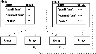For example, this sharing allows members of a time series, defined on a fixed grid and represented by two Fields, to share positions and connections while each has different data.

In addition, sharing is vital to an efficient implementation of the data flow programming model, in which a module may not modify its inputs. In the example in Figure 3, the first Field might represent the input to a module (e.g., a vector Field), while the second Field might represent the output from a module that computes the length of each vector. The module has constructed a Field with a separate "data" component representing the calculated result, but has not had to copy the portions of the Field that remained the same (positions and connections), because they could be shared between the input and output Fields.

Standard Components

Table 1. Standard Field Components

Component	Type	Meaning
"data"	arbitrary	user's data (dependent variable)
"positions" "invalid positions"	float[n] char	n-space sample points which sample points are invalid
"colors" "colors" "color map" "front colors" "back colors" "opacities" "opacities" "opacity map"	float[3] char float[3] float[3] float[3] float char float	surface or volume colors color index (see "color map") color map indexed by "colors" component colors of front of surface colors of back of surface opacity of surface or volume opacity index (see "opacity map") opacity map indexed by "opacities" component
"tangents" "normals" "binormals"	float[3] float[3] float[3]	curve tangent curve or surface normal second curve normal
"connections" "invalid connections"	int[k] char	interpolation elements which interpolation elements are invalid
"faces" "loops" "edges"	int int int	faces described as a collection of loops loops described as a series of edges edges described as a series of points
"pick" "paths" "pickpaths"		picks paths pickpaths
"neighbors" "box" "data statistics"	int[p] float[2n]	pointers to connection neighbors 2n corners of a bounding box statistics for data component

Positions Component

The "positions" component is an Array Object specifying a set of n-dimensional positions. For data on a grid with regular positions, the positions can be encoded compactly by Regular and Product Arrays, which are described in "Arrays".

Connections Component

The "connections" component provides a means for interpolating data values between the positions. Each item of the "connections" Array describes an interpolation element such as a line, triangle, tetrahedron or cube. The vertices of each such interpolation element are specified by one Array item consisting of a list of indices into the "positions" Array, one index per vertex of the interpolation element. (Position index numbers begin at 0.)

The type of the interpolation elements is specified by the "element type" attribute of the "connections" component. Two open-ended series of element types are currently defined: the n-dimensional simplexes, and the n-dimensional cuboids.

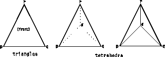
The n-dimensional simplexes are represented by "connections" components with "element type" attributes of "triangles" (2-D) or "tetrahedra" (3-D). Each item of such a "connections" component is a list of n+1 integer indices referring to items in the "positions" component representing the n+1 vertices of an n-dimensional simplex. These vertices are ordered as illustrated in Figure 4. For tetrahedra, the parity of all tetrahedra in a given Field must be consistent. Figure 4 illustrates the two possible parities for tetrahedra. In addition, for triangles there is a convention for which face is the front (using the right-hand rule).

Figure 4. Order of Vertices in Triangles and Tetrahedra. In the tetrahedron at right, s is the point nearest the viewer; at center, the point furthest from the viewer.

The n-dimensional cuboids are represented by "connections" components with "element type" attributes of "lines" (1D), "quads" (2-D), "cubes" (3-D), "cubes4D", and so on in the format "cubesnD", where n represents the number of dimensions. Each item of such a "connections" component is a list of 2ⁿ integer indices referring to items in the "positions" component representing the 2ⁿ vertices of an n-dimensional cuboid. The ordering of these vertices is illustrated in Figure 5. For cubes, the parity of all cubes in a given Field must be consistent. In addition, for quads there is a convention that determines the front face.

Figure 5. Order of Vertices in Quads and Cuboids

Note:

Figure 5 does not indicate the correspondence between the edges of the cubes or quads and the spatial dimensions. For example, the cubes or quads can be "irregular," in which case the positions of each vertex are specified explicitly. Regular "positions" components can specify an arbitrary correspondence between the spatial dimensions and the edges of the cube, as illustrated in Figure 10.

For data on grids with regular connections, the connections can be encoded compactly by Path and Mesh Arrays, which are described in "Arrays" and in more detail in Appendix B. "Importing Data: File Formats".

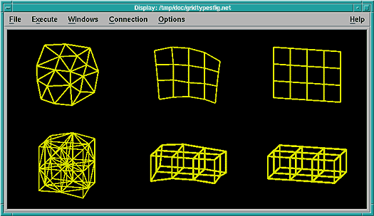
Figure 6 illustrates the various types of grids formed with different kinds of "positions" and "connections" components.

Figure 6. Examples of Grid Types. The three grids in the top row represent surfaces; those in the bottom row, volumes. Reading from left to right, the three grid types are: irregular (irregular positions, irregular connections), deformed regular (irregular positions, regular connections), and regular (regular positions, regular connections).

Data Component

The "data" component stores the user's data values. The data values can be position- or connection-dependent, as specified by the value of the "dep" attribute (described in "Standard Attributes") of the "data" component. If the values are position-dependent, then the "connections" component supplies a means of interpolating data values between the samples. If the values are connection-dependent, the data value is constant for each interpolation element. Data can also be dependent on "faces" or "polylines" (see "Edges and Polylines"), in which case the data is constant for either the face or the polyline.

The data are in one-to-one correspondence with the component upon which they are dependent. This means that they are specified in the same order as the items in the corresponding component. If that component is specified in a compact form, its contents are ordered as described in "Arrays".

Colors, Front Colors, and Back Colors Components

The "colors", "front colors", and "back colors" components are a means of specifying another, specialized type of dependent data. Specifically, the renderer requires that each object in a scene have at least one of these components. The "front colors" and "back colors" components specify colors to be associated with the front and back sides, respectively, of a surface. The "colors" component specifies colors to be associated with both sides of a surface, or with a volume. If only "front colors" or only "back colors" are specified, then only the "front" or "back" sides, respectively, of the polygons are rendered. If present, "front colors" or "back colors" override the specification of the "colors" component.

Each item of a color component Array consists of three floating-point numbers specifying the red, green, and blue component of a color respectively. The color components can use the entire floating-point range, but by convention the range from 0 to 1 is mapped onto the available range of the output device. Like the "data" component, the color components can be position- or connection-dependent.

The front of a triangle is defined to be the side such that the path traversing the vertices in the order that they are listed for the triangle appears to go counterclockwise. The front of a quad is the side from which the vertex numbering appears (Figure 5).

The interpretation of colors differs between surfaces and volumes. For surfaces, the color values in the range from 0 to 1 are mapped onto the range of colors values possible for the display. For volumes, the interpretation of colors follows the "dense emitter" model described in the next section.

Opacities Component

The "opacities" component plays a role similar to that of colors components, except that it specifies a floating-point opacity for rendering. Its interpretation differs depending on whether the connections represent a surface (triangles or quads), or a volume (tetrahedra, cubes, and so on). In the surface case, the opacity is a number from 0 to 1 specifying the opacity of the surface. In the volume case, the opacity represents the instantaneous attenuation of light per unit distance traveled. Like the colors components, it can be position- or connection-dependent.

The interpretation of "colors" and "opacities" differs between surfaces and volumes. For surfaces, a surface of color c_f and opacity o is combined with the color c_b of the objects behind it resulting in a combined color c_fo + c_b(1 - o).

For volumes, the "dense emitter" model is used, in which the opacity represents the instantaneous rate of absorption of light passing through the volume per unit thickness, and the color represents the instantaneous rate of light emission per unit thickness. If c(z) represents the color of the object at z and o(z) represents its opacity at z, then the total color of a ray passing through the volume is given by:

Color Map and Opacity Map Components

There is an alternative to having the "colors" component and "opacities" component explicitly list the color and opacity associated with each position or connection element. If each element of the "colors" and "opacities" components is a single byte, then it is interpreted as an index into the "color map" or "opacity map" component. The "color map" component is a 256-element table of three floating-point values (representing red, green, and blue, typically with values between 0 and 1). The "opacity map" component is a 256-element table of floating-point values between 0 and 1.

Invalid Positions and Invalid Connections Components

The "invalid positions" and "invalid connections" components allow positions or connections to be marked as not having valid data. This is useful, for example, for observational data defined on a regular grid but with occasional missing observations, or for simulation data defined on a regular grid but with a "hole" covered by another grid, perhaps at a higher resolution. The "invalid positions" component can be an Array of bytes or unsigned bytes, one for each position, where the component is dependent on positions (i.e., has a "dep" attribute of "positions."). In that case, the value 1 indicates that the corresponding position is invalid, and 0 that the corresponding position is valid. Alternatively, the "invalid positions" component can be an Array of signed or unsigned integers, where the component references the positions (i.e., has a "ref" attribute of "positions"). In that case, the component contains a list of the indices of the invalid positions. The first method is more space-conserving when there are a large number of invalid elements; the second, when there are a relatively small number. See Compute in IBM Visualization Data Explorer User's Reference for a way to convert from the "ref" type to the "dep" type.

The "invalid connections," "invalid faces," and "invalid polylines" components can be defined in an analogous way.

Tangents, Normals, and Binormals Components

The "normals" component is used to specify a local surface normal for rendering purposes. The "tangents", "normals" and "binormals" components specify a local reference frame on a path; this is useful, for example, for twisted-ribbon representations of streamlines.

Normals are used for, among other things, surface shading. By convention, the normals are expected to point out from the front of a surface, as defined in "Colors, Front Colors, and Back Colors Components". Normals are expected to have unit length.

Neighbors Component

The "neighbors" component represents information about the neighbors of each connection element. The number of items in this component must match the number of items in the "connections" component. The number of entries in each item must match the number of faces (for 3-D) or edges (for 2-D) in the connection element. For example, each item in the "neighbors" component for triangle connections has three entries, while each item in the "neighbors" component for tetrahedral connections has four entries.

For simplexes in n dimensions (for example, triangles and tetrahedra), each item of the neighbors Array consists of n+1 integer indices into the connections Array identifying the n+1 neighbors of the simplex; the ith of the n+1 indices corresponds to the face opposite the ith vertex of the simplex. For quads, cubes, and so on, each item of the neighbors Array contains 2n integer indices into the connections Array identifying the 2n neighbors of the polyhedron. The pointers are in the order -x₁+x₁-x₂+x₂ ... -x_n+x_n, meaning that the first index points to the neighbor in the -x₁ direction, the second to the neighbor in the +x₁ direction, and so on, where the x_n dimension varies fastest in the representation of the point indices in the interpolation element. Faces without neighbors are indicated by an index of -1.

Box Component

The "box" component consists of 2ⁿ n-dimensional points, where n is the dimensionality of the positions component, identifying the corners of a bounding box that contains the positions of this Field.

Data Statistics Component

The "data statistics" component contains statistics of the "data" component. The information in this component should be accessed using the Statistics module or the DXStatistics() function, as the exact contents are undefined. If DXStatistics is called on other components (e.g., "positions"), an analogous component (in this case "positions statistics") will be created.

Faces, Loops, and Edges Components

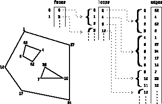
The "faces", "loops", and "edges" components are used for special-purpose applications, such as fonts or geometric models. The "faces" component represents a set of faces, each described as a set of loops. Each entry in the face Array is a single integer index into the "loops" Array identifying the first of a consecutive set of loops for this face. The loops are listed in order of the faces they are associated with, so that the list of loops for face i ends in the loops Array just before the first loop for face i+1. Each entry in the "loops" Array is a single integer index into the "edges" Array, identifying the first of a consecutive set of edges for this loop. The edges are listed in order of the loops they are associated with, so that the list of edges for loop i in the edges Array ends just before the first edge for loop i+1. Each entry in the edges Array is a single integer index into the "points" Array identifying one vertex of an edge; the other vertex of an edge is the next entry in the "edges" Array, except that the last edge in a loop that connects the last point to the first point is not listed explicitly. This is illustrated in Figure 7.

Figure 7. Use of Faces, Loops, and Edge Components

If you can guarantee that the first loop for each face is an enclosing loop, and that any subsequent loops, are completely enclosed holes in the face, then you may be able to increase performance when processing faces, loops, and edges data by setting the DX_SIMPLE_LOOPS environment variable (see "Other Environment Variables"). However, setting this environment variable may cause the executive to crash if data is not conformant.

Edges and Polylines

"Polylines" are a way of collecting a set of line segments into a single object with which data can be associated. They are implemented much as faces, loops, and edges are (see above). An "edges" component contains the indices of the vertices along polylines. A "polylines" component contains the indices of the first element in the "edges" component of each polyline sequence. In other words, the i^th element of the "polylines" component is the index in the "edges" component at which the sequence of vertex indices of polyline i starts. The sequence corresponding to polyline[i] continues to the beginning of the next polyline sequence (or to the end of the "edges" component). Polyline data may be dependent on either "polylines" or "positions".

Pokes, Picks, and Pick Paths Components

The pokes, picks, and pick paths components are created as part of the picking process, as implemented by the Pick tool. A user writing a module that uses the pick structure output by the Pick tool is expected to use the pick structure manipulation routines (as described in IBM Visualization Data Explorer Programmer's Reference) rather than accessing the pick structure directly. The contents of the pick structure are not defined.

Standard Attributes

The standard defined attributes are listed in Table 2 and Table 3, and are further described in the subsequent paragraphs. Attributes associated with rendering properties are described under the Display module in Chapter 1. "Data Explorer Tools" in IBM Visualization Data Explorer User's Reference.

Table 2. Component attributes

Attribute	Meaning
"dep"	component that this component depends on
"ref"	component that this component refers to
"der"	component that this component is derived from
"element type"	interpolation method for connections component

Table 3. Object attributes

Object	Relevant module
label	Plot
scatter	Plot
mark	Plot
mark every	Plot
mark scale	Plot
fuzz	Display, Render, Image
ambient	Display, Render, Image
diffuse	Display, Render, Image
specular	Display, Render, Image
shininess	Display, Render, Image
shade	Display, Render, Image
opacity multiplier	Display, Render, Image
color multiplier	Display, Render, Image
texture	Display, Image
direct color map	Display
cache	Display, Image
rendering mode	Display, Image
rendering approximation	Display, Image
render every	Display, Image
pickable	Pick
marked component	Mark, Unmark

dep Attribute

The "dep" attribute specifies which component the given component depends on. The dependent component is specified by a String Object naming the component it depends on. For example, if the data is position-dependent, it has a "dep" attribute that is a String Object naming the "positions" component. A component with a this attribute is expected to be in a one-to-one correspondence with the component named in the attribute.

ref Attribute

The "ref" attribute specifies which component the given component refers to. The referent component is specified by a String Object naming the component it refers to. For example, the "connections" component generally has a "ref"attribute that is a String Object naming the "positions" component. A component with this attribute consists of indices into the component named in the attribute.

der Attribute

The "der" attribute specifies that a component is derived from another component, and so should be recalculated or deleted when the component it is derived from changes. For example, the "box" component has a "der" attribute that is a String Object naming the "positions" component.

element type Attribute

The "element type" attribute is an attribute of the "connections" component. It is a String Object naming the type of the interpolation primitives. See "Connections Component" for a list of the possible values of the "element type" attribute.

label, scatter, mark, mark every, mark scale Attributes

fuzz, ambient, diffuse, specular, shininess, shade Attributes

opacity multiplier, color multiplier Attributes

texture Attribute

direct color map Attribute

cache Attribute

rendering mode Attribute

rendering approximation, render every Attributes

pickable Attribute

marked component Attribute

Arrays

Array Objects hold the actual data, positions, connections, and so on. An Array consists of some number of items numbered consecutively starting at 0. Each item has a type, category, rank and shape, defined as follows:

Type	Types include double, float, int, uint, short, ushort, byte, ubyte, and string. (For example, byte is signed byte and ubyte is unsigned byte.)
Category	A category can be real or complex.
Rank	Rank 0 corresponds to scalars, rank 1 to vectors, rank 2 to matrices or rank-2 tensors; higher ranks correspond to higher-order tensors.
Shape	The shape is defined as the list of dimensions of the structure. For rank-0 items (scalars), there is no shape. For rank-1 structures (vectors), the shape is a single number corresponding to the number of dimensions. For rank-2 structures, shape is two numbers, and so on.

The following are examples of these classifications:

• Three-dimensional points have type float or double, category real, rank 1, and shape 3.
• Two-vectors typically have type float. They are category real, rank 1, and shape 2. Three-vectors are shape 3.
• Tetrahedra have type int, category real, rank 1, and shape 4.
• Scalar values typically have type int or float. They are category real and rank 0, with no shape.
• Strain tensors typically have type float or double. They are category real, rank 2, and shape 3×3.

The Array types are discussed in the following sections.

Irregular Arrays

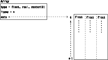
The most general way to specify the contents (item values) of an Array is to list the values; this is called irregular data. An example of such an Array Object is illustrated in Figure 8.

Figure 8. Example of an Irregular Array

Regular Array

A set of n-dimensional points lying on a line in n-space with a constant n-dimensional delta between them, represents, for example, one edge of a grid of regular positions. Regular Arrays are frequently combined as the terms of a Product Array. An example of a Regular Array is illustrated in Figure 9.

This example represents (in compact form) the same information as the following irregular Array:

[ x_o ,   y_o ]
[ x_o + x_d , y_o + y_d ]
[ x_o + 2x_d , y_o + 2y_d ]
.
.
.
[ x_o + (n - 1) x_d , y_o + (n - 1) y_d ]

Figure 9. Example of a Regular Array

type = float, real, vector[2] items = n origin = [xo, yo] delta = [xd, yd]

Product Array

Encodes multidimensional positional regularity. It is the set of points obtained by summing one point from each of the terms of the product in all possible combinations. For example, the product of a set of Regular Arrays is a regular grid whose basis vectors are the deltas of the Regular Arrays that are the terms of the product, and whose origin is the sum of the origins of the terms. An example of a Product Array Object is illustrated in Figure 10. A Product Array can have terms that are Regular Arrays, irregular Arrays, or any combination of Regular and irregular Arrays.

Figure 10. Example of a Product Array

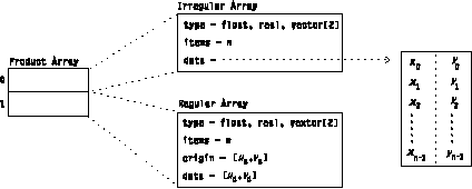The example in Figure 10 represents (in compact form) the same information as the following irregular Array:
[ x_o + u_o , y_o + v_o ]
[ x_o + u_o + u_d , y_o + v_o + v_d ]
[ x_o + u_o + 2u_d , y_o + v_o + 2v_d ]
.
.
.
[ x₁ + u_o , y₁ + v_o ]
[ x₁ + u_o + u_d , y₁ + v_o + v_d ]
.
.
.
[ x_{<n - 1>} + u_o + (m - 1) u_d , y_{<n - 1>} + v_o + (m - 1) v_d ]

An important special case of the more general Product Array Object is the n-dimensional geometrically regular grid. Figure 11 is an example that shows two ways to describe a Product Array composed of two Regular Arrays.

Figure 11. Product Array of Two Regular Arrays

The order of the specification of the counts and deltas implicitly creates a list of positions. x is the fastest-varying dimension. This represents (in compact form) the same information as the following irregular Array: [0 0] [1 0] [2 0] [3 0] [0 1] [1 1] [2 1] · y is the fastest-varying dimension. This represents (in compact form) the same information as the following irregular Array: [0 0] [0 1] [0 2] [1 0] [1 1] [1 2] [2 0] ·

Path Array

Encodes linear regularity of connections. It is a set of n-1 line segments joining n points, where the ith line segment joins points i and i+1. Path Arrays are frequently combined as the terms of a Mesh Array. An example of a Path Array is illustrated in Figure 12.

Figure 12. Example of a Path Array

type = int, real, vector[2] items = n

This example represents (in compact form) the same information as the following irregular Array:
[ 0   1 ]
[ 1   2 ]
[ 2   3 ]
.
.
.
[ n - 2   n - 1 ]

Mesh Array

Encodes multidimensional regularity of connections. It is a product of connection Arrays. The product is a set of interpolation elements where the product has one interpolation element for each pair of interpolation elements in the two multiplicands, and the number of sample points in each interpolation element is the product of the number of sample points in each of the multiplicands' interpolation elements. An example of a Mesh Array is illustrated in Figure 13.

Figure 13. Example of a Mesh Array
This example represents (in compact form) the same information as the following irregular Array:

[ 0 , 1 , m , m + 1 ] [ 1 , 2 , m + 1 , m + 2 ] . . . [ m - 2 , m - 1 , 2m - 2 , 2m - 1 ] [ m , m + 1 , 2m , 2m + 1 ] . . .

An important special case of the more general Mesh Array Object is the n-dimensional cuboidal connections of a regular grid. Figure 14 is an example that shows a Mesh Array composed of two Path Arrays.

See Appendix B. "Importing Data: File Formats" for a detailed description of how to specify these compact Arrays.

Figure 14. Mesh Array of Two Path Arrays (with Regular Connections)

The order of the specification of the counts implicitly creates a list of position indices in the order of "last index varies fastest." The location in space of each vertex is determined by the value of the position referred to by that index. This represents (in compact form) the same information as the following irregular Array: [ 0   1   3   4 ] [ 1   2   4   5 ] [ 3   4   6   7 ] · This represents (in compact form) the same information as the following irregular Array: [ 0   1   5   6 ] [ 1   2   6   7 ] [ 2   3   7   8 ] ·

Constant Array

Encodes a set of numbers all with the same value. This can be useful, for example, for specifying the colors associated with an object if the object has a single color. An example of a Constant Array is shown in Figure 15.

Figure 15. Example of a Constant Array

type = float, real, vector[3] items = n origin = [xo, yo, zo]

Groups

Fields can be combined into Groups. A Group is a collection of members that themselves may be Fields or other Groups. A member can be referred to either by name or by index. An example of a Group is given in Figure 16.

Figure 16. Example of a Group

This example shows a Group describing a visualization scene composed of two parts. The member named "pressure" is a Field of volumetric data to be volume rendered, representing pressure in an airflow around an airplane. The member named "airplane" is a geometric model describing the surface of the airplane. It, in turn, can be a Group, where each member is one of the constituent parts of the airplane, such as "wing," "fuselage," and so on. The top-level Group could then be passed into the renderer to produce an image of the airplane combined with a volume rendering of the pressure Field.

Named Group members can be retrieved by name or by index number; the n members of a Group are numbered from 0 to n-1. Group members can also be stored by index number without a name, in which case they can be retrieved only by index number. The members of a Group are always numbered consecutively starting at 0, and gaps in the numbering are not allowed.

In addition to generic Groups used to collect related information, there are three subclasses of Group used to combine related Objects with additional semantics: Multigrid Groups, Composite Field Groups, and Series Groups.

Multigrid Groups

It is often necessary to represent a Field as a collection of separate Fields, each with its own grid. For example, this is the case in some kinds of simulations using multiple grids. The data structure used to hold such Fields is a subclass of Group called a Multigrid Object. It is the same as a generic Group in most respects, except that it requires all members to be Fields holding data of the same type. The "connections" component of each member must also be of the same type. Grids may be completely disjoint or may overlap. For overlapping grids, the "invalid positions" or "invalid connections" components may be used to define which grid is valid in a particular region.

Composite Field Groups

A Composite Field is another kind of Group that is treated as a single entity. For example, parallelism in Data Explorer is achieved by explicitly partitioning Fields into abutting, spatially disjoint primitive Fields. Positions on the boundaries must be replicated identically. Like Multigrid Groups, all members must have the same type of data and the same type of connections.

Series Groups

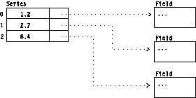
Series of various types, such as time series, are stored in a subclass of Group called a Series Object. A Series Object is the same as a generic Group in most respects, except that it associates a series value, such as a time stamp, with each member. Members are stored in and retrieved from a Series Group by index. Members cannot be retrieved by series value. Fields in a Series Group must all have the same data type and connection element type.  Figure 17 shows an example of a Series Group, where the three members have series positions of 1.2, 2.7, and 8.4 respectively.

Figure 17. Example of a Series Group